Reinforcement learning is an area of machine learning concerned with the behaviour of an agent in an environment, whose goal is to interact with the environment in order to maximize some type of reward. This general idea can be applied to solve a wide range of tasks, from winning at chess to beating the world champion of Go, from teaching a robot how to move to designing new drugs. In this article, we will cover part of the theoretical foundations of reinforcement learning, starting with Markov Decision Processes (MDPs) and value functions. These will give us a foundation for treating reinforcement learning problems in general.
To speak concretely about Reinforcement Learning, we fist need to define Markov Decision Processes (MDPs). Wikipedia states that MDPs provide a mathematical framework for modeling decision making in situations where outcomes are partly random and partly under the control of a decision maker.
We will see what this means in detail later on. The important thing to understand is that MDPs formally describe an environment for RL. The agent will interact with such environment, guided by the rewards it gets along the way.

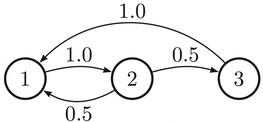
The basic entities of MDPs are its states. A state in an MDP is called a Markov state, meaning that a particular state captures all relevant information from history. Once we know a state, history can be thrown away.
\[ \begin{align*} P[S_{t+1} \mid S_t] = P[S_{t+1} \mid S_1,S_2,...,S_t] \end{align*}\]
In addition to a set of states, we also need to define the state transition probabilities. A state transition probability defines the probability of going from state s to state s'.
\[ \begin{align*} \textit{P}_{ss'} = P[S_{t+1} = s' \mid S_t = s] \end{align*}\]
As a more compact way of representing such probabilities, we define the state transition matrix P.
\[ \begin{align*} \textit{P} = \begin{bmatrix} P_{11} & \dots & P_{1n} \\\ \vdots \\\ P_{n1} & \dots & P_{nn} \end{bmatrix} \end{align*}\]
This matrix defines the transition probability for each possible pair of states. Given the elements we just defined, we can now define a generic Markov process, also called Markov Chain:
\[ \begin{align*} \text{A Markov process is a tuple } \langle S,P \rangle \text{ in which: } \end{align*}\]
- $S$ is a set of states.
- $P$ is a state transition probability matrix.

If we add only two more ingredients to out Markov Process, we get a Markov Reward Process.
As you can guess, one of these elements is a Reward Function. A Reward Function represents a very simple thing: for each state in our process, it tells us the expected value of the reward in that state.
\[ \begin{align*} R_s = E[R_{t+1} \mid S_t = s] \end{align*}\]
The second elements is more subtle: it's the discount factor.
\[ \begin{align*} \gamma \in [0,1] \end{align*}\]
The discount factor, as you will see, is used to decrease the value of rewards in the future. We are now ready to define our return $G_t$.
\[ \begin{align*} G_t = R_{t+1} + \gamma R_{t+1} + ... = \sum_{k=0}^{\infty} \gamma^k R_{t+1+k} \end{align*}\]
As you can see, the return is nothing but the total discounted reward from time-step t.
Most Markov Reward Process are discounted and there are several reasons to this. Mainly, discounting rewards allows us to represent uncertainty about the future, but it also helps us model human behaviour better, since it has been shown that humans/animals have a preference for immediate rewards.
Also, the math is easier if we use discount factors, and we are able to avoid infinite returns in cyclic processes.
We are now ready to define one of the most important functions in Reinforcement Learning: the value function, also called state value function.
The value function of a MRP is the expected return starting from state S.
\[ \begin{align*} v(s) = E[G_t \mid S_t = s] \end{align*}\]
This function can be decomposed into two parts:
- immediate reward $R_{t+1}$
- discounted value of successor state $\gamma v(S_{t+1})$, as follows:
\[ \begin{align} v(s) & = E[G_t \mid S_t = s] = E[R_{t+1} + \gamma R_{t+2} + \gamma^2 R_{t+3} + \ldots \mid S_t = s] \\ & = E[R_{t+1} + \gamma (R_{t+2} + \gamma R_{t+3} + \ldots) \mid S_t = s] \\ & = E[R_{t+1} + \gamma G_{t+1} \mid S_t = s] \\ & = E[R_{t+1} + \gamma v(S_{t+1}) \mid S_t = s] \\ \end{align}\]
This formula for the value function takes the name of Bellman equation. It is of fundamental importance because it allows us to have a recursive representation of the value function. This property is important in practice, when we need to implement ways of computing/evaluating/maximizing this function.
The Bellman equation can also be expressed using matrices.
\[ \begin{align*} v = R + \gamma P v \end{align*}\]
where $v$ is a column vector with one entry per state.
\[ \begin{align*} \begin{bmatrix} v(1) \\\ \vdots \\\ v(n) \end{bmatrix} = \begin{bmatrix} R_1 \\\ \vdots \\\ R_n \end{bmatrix} + \gamma \begin{bmatrix} P_{11} & \dots & P_{1n} \\\ \vdots \\\ P_{n1} & \dots & P_{nn} \end{bmatrix} \begin{bmatrix} v(1) \\\ \vdots \\\ v(n) \end{bmatrix} \end{align*}\]
The Bellman Equation is linear, which means that we can solve it directly. However, the computational complexity is $\mathcal{O}(n^3)$, which makes it unfeasible to compute for big MRPs with many states.
Therefore, in practice, iterative methods are used, such as Dynamic Programming, Monte-Carlo evaluation, and Temporal Difference. We will see these methods in detail in future posts of these series.
We are now ready to add our last ingredient to have a complete MDP: a set of Actions A.
Le't sum it up: a Markov Decision Process is a tuple $\langle S,A,P,R,\gamma \rangle$
- $S$ is a finite set of states
- $A$ is a finite set of actions
- $P$ is a state transition probability matrix $\textit{P}_{ss'}^a = P[S_{t+1} = s' \mid S_t = s, A_t = a]$
- $R$ is a reward function $ R_s^a = E[R_{t+1} \mid S_t = s, A_t = a]$
- $\gamma$ is a discount factor $\gamma \in [0,1]$
Now that we have our MDP, we can define the behaviour of an agent in this environment. We define the agent's behaviour with a policy $\pi$, which is simply a distribution over actions given states. It basically maps states to the probabilities of our agent taking each possible action from that state.
Simple, right?
\[ \begin{align*} \pi (a \mid s) = P[A_t = a \mid S_t = s] \end{align*}\]
We can now rewrite our value function, when we follow policy $\pi$:
\[ \begin{align*} v_{\pi}(s) = E_{\pi}[G_t \mid S_t = s] \end{align*}\]
This equation represents the expected return starting from state $s$, and following policy $\pi$.
Another important function in RL, called action-value function, expresses the expected value of first taking a certain action, and then following a certain policy.
\[ \begin{align*} q_{\pi}(s,a) = E_{\pi}[G_t \mid S_t = s, A_t = a] \end{align*}\]
Again, we can rewrite our value function in the Bellman form:
\[ \begin{align*} v_{\pi}(s) = E_{\pi}[R_{t+1} + \gamma v_{\pi}(S_{t+1}) \mid S_t = s] \end{align*}\]
And we can write the action-value function in a similar fashion:
\[ \begin{align*} q_{\pi}(s,a) = E_{\pi}[R_{t+1} + \gamma q_{\pi}(S_{t+1}, A_{t+1}) \mid S_t = s, A_t = a] \end{align*}\]
The optimal state-value function $v*(s)$ is the maximum value function over all policies.
\[ \begin{align*} v*(s) = \max_{\pi} v_{\pi}(s) \end{align*}\]
Similarly, the optimal action-value function is the maximum action-value function over all policies.
\[ \begin{align*} q*(s,a) = \max_{\pi} q_{\pi}(s,a) \end{align*}\]
We say that an MDP is solved when we find the optimal value function.
Daniele is a computer engineering graduate student in Turin, focusing on data science and machine learning. He graduated from his bachelor with a thesis on generative models. He also organises the Machine Learning study group in Turin. Previously, he worked as a software engineer, and presented his projects at Tel Aviv University and Google Tel Aviv. He was also selected to participate in the first edition of CyberChallenge.it.
If you liked our article, remember that subscribing to the Italian Association for Machine Learning is free! You can follow us daily on Facebook, LinkedIn, and Twitter.