Variational Autoencoders 1 - The Basics

The Variational Autoencoder (VAE) is a not-so-new-anymore Latent Variable Model (Kingma & Welling, 2014), which by introducing a probabilistic interpretation of autoencoders, allows to not only estimate the variance/uncertainty in the predictions, but also to inject domain knowledge through the use of informative priors, and possibly to make the latent space more interpretable. VAEs can have various applications, mostly related to data generation (for example, image generation, sound generation and missing data imputation)¹.

\[ \DeclareMathOperator\supp{supp} \DeclareMathOperator*{\argmax}{arg\,max}\]

VAEs are generative models

Unlike classical (sparse, denoising, etc.) autoencoders, VAEs are probabilistic generative models, like GANs (Generative Adversarial Networks). With generative we denote a model which learns the probability distribution $p(\mathbf{x})$ over the input space $\mathcal{X}$. This means that after training such a model, we can then sample from our approximation of $p(\mathbf{x})$. If our training set contains handwritten digits (MNIST), then the trained generative model is able to create images which look like handwritten digits, even though they're not "copies" of the images in the training set. In the case of images, if our training set contains natural images (CIFAR-10) or celebrity faces (CelebA), it will generate images which look like photo pics.

Learning the distribution of the images in the training set implies that images which look like handwritten digits (for example) have an high probability of being generated, while images which look like the Jolly Roger or random noise have a low probability. In other words, it means learning about the dependencies among pixels: if our image is a $28\times 28=784$ pixels grayscale image from MNIST, the model should learn that if a pixel is very bright, then there's a significant probability that some neighboring pixels are bright too, that if we have a long, slanted line of bright pixels we may have another smaller, horizontal line of pixels above this one (a 7), etc.

VAEs are Latent Variable models

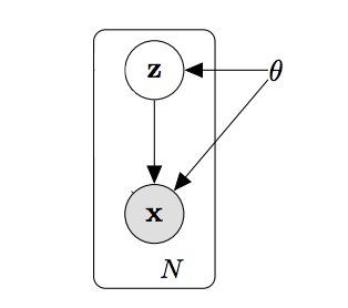
The VAE is a Latent Variable Model (LVM): this means that $\mathbf{x}$, the random vector of the 784 pixel intensities (the observed variables), is modeled as a (possibly very complicated) function of a random vector $\mathbf{z}\in\mathcal{Z}$ of lower dimensionality, whose components are unobserved (latent) variables. Usually an uncorrelated Gaussian prior for $\mathbf{z}$ is assumed, but this is not required. Coincisely, we assume the following data generating process:

\[ \begin{align} \mathbf{z} &\sim p_{\theta^*}(\mathbf{z}) \\ \mathbf{x}\vert\mathbf{z} &\sim p_{\theta^*}(\mathbf{x}\vert\mathbf{z}) \end{align}\]

And we assume that both the prior $p_{\theta^*}(\mathbf{z})$ and the likelihood $p_{\theta^*}(\mathbf{x}\vert\mathbf{z})$ come from some parametric families (possibly different). The corresponding DAG (Directed Acyclic Graph) is then:

Latent variable models are also sometimes called hierarchical or multilevel models, and they are models that use the rules of conditional probability to specify complicated probability distributions over high dimensional spaces, by composing simpler probability density functions. The original VAE has only two levels, but recently an amazing paper on a hierarchial VAE with multiple levels of latent variables has been published (note that the hierarchy of latent variables in a probabilistic model has nothing to do with the layers of a neural network).

When does a latent variable model make intuitive sense? For example, in the MNIST case we think that the handwritten digits belong to a manifold of dimension much smaller than the dimension of $\mathbf{x}$, because the vast majority of random arrangements of 784 pixel intensities, don't look at all like handwritten digits. The representation of the image should be equivariant to certain transformations (e.g., rotations, translations and small deformations) but not to others. So in this case it makes sense to think that the image samples are generated by taking samples (which we don't observe) in a sample space of much smaller dimension, and then transforming them according to some complicated function.

Estimating the model

We are now given a dataset consisting of $N$ i.i.d. samples, $\mathbf{X}=\{\mathbf{x}_i\}_{i=1}^N$ (note again that we do not observe $\mathbf{z}$) and we want to estimate $\theta^*$. The standard "recipe" would be to maximize the likelihood of the data (marginalized over the latent variables), i.e., Maximum Likelihood Estimation:

\[ \hat{\theta}=\argmax_{\theta\in\Theta}p_{\theta}(\mathbf{X}) =\argmax_{\theta\in\Theta}\sum_{i=1}^N\log_{\theta}{p(\mathbf{x}_i)}\]

However, we're immediately faced with two challenges:

1. computing $p_{\theta}(\mathbf{x}_i)$ requires solving the integral

   \[ p_{\theta}(\mathbf{x}_i) = \int p_{\theta}(\mathbf{x}_i\vert\mathbf{z})p_{\theta}(\mathbf{z})d\mathbf{z} \label{a}\tag{1}\]

   which is often intractable ², even in the simple case of one hidden layer nonlinear neural networks.

2. we need to compute the integral for all $N$ data samples $\mathbf{x}_i$ of a large dataset, which rules out either batch optimization, or sampling-based solutions such as Monte Carlo EM, which would require an expensive sampling step for each $\mathbf{x}_i$.

We need to get waaay smarter.

Enter Variational Inference

To solve the first problem, i.e., the intractability of the marginal likelihood, we use an age-old (in ML years) trick: Variational Inference (introduced in Jordan et al., 1999 and nicely reviewed in Blei et al., 2018). VI transforms the inference problem into an optimization problem. This way, we get rid of integration, but we pay a price, as we'll see later. Fair warning: this section is more mathy than the rest. I'll introduce necessary concepts such as the Kullback-Leibler divergence, but you may want to skip to the next session, for a first read.

The Kullback-Leibler divergence

VI starts by introducing a family $\mathcal{Q}$ of parametric approximations $q_{\phi}(\mathbf{z}\vert\mathbf{x})$ to the true posterior distribution $p_{\theta}(\mathbf{z}\vert\mathbf{x})$, indexed by $\phi$. The goal of VI is to find the value(s) of $\phi$ such that $q_{\phi}(\mathbf{z}\vert\mathbf{x})\in\mathcal{Q}$ is "closest" to $p_{\theta}(\mathbf{z}\vert\mathbf{x})$ in some sense. In particular, we seek to minimize the Kullback-Leibler divergence

\[ D_{KL}(q_{\phi}(\mathbf{z}\vert\mathbf{x})\vert\vert p_{\theta}(\mathbf{z}\vert\mathbf{x}))=\int q_{\phi}(\mathbf{z}\vert\mathbf{x}) \log{\frac{q_{\phi}(\mathbf{z}\vert\mathbf{x})}{p_{\theta}(\mathbf{z}\vert\mathbf{x})}}d\mathbf{z} \]

which is a similarity measure for probabilities distributions. For the following, we'll need two properties of $D_{KL}$:

1. $D_{KL}(q\vert\vert p)\ge0 \ \forall p,q$
2. $D_{KL}(q\vert\vert p) = 0 \iff p = q \ \text{a.e.}$

Some ELBO grease

However, our primary goal is to estimate the generative model parameters $\theta^*$ through Maximum (Marginal) Likelihood Estimation. Thus, let's try to rewrite the marginal log-likelihood of a data point in terms of $D_{KL}(q_{\phi}(\mathbf{z}\vert\mathbf{x}_i)\vert\vert p_{\theta}(\mathbf{z}\vert\mathbf{x}_i))$:

\[ \begin{multline}\log{p_{\theta}(\mathbf{x}_i)} = \log{p_{\theta}(\mathbf{x}_i)}\int q_{\phi}(\mathbf{z}\vert\mathbf{x}_i)d\mathbf{z} = \int q_{\phi}(\mathbf{z}\vert\mathbf{x}_i)\log{p_{\theta}(\mathbf{x}_i)} d\mathbf{z} = \\ \int q_{\phi}(\mathbf{z}\vert\mathbf{x}_i)\log{\frac{p_{\theta}(\mathbf{x}_i, \mathbf{z})}{p_{\theta}(\mathbf{z}\vert\mathbf{x}_i)}} d\mathbf{z} = \int q_{\phi}(\mathbf{z}\vert\mathbf{x}_i) \log{\frac{p_{\theta}(\mathbf{x}_i, \mathbf{z})}{p_{\theta}(\mathbf{z}\vert\mathbf{x}_i)}\frac{q_{\phi}(\mathbf{z}\vert\mathbf{x}_i)}{q_{\phi}(\mathbf{z}\vert\mathbf{x}_i)}} d\mathbf{z} \end{multline}\]

where in the second-to-last inequality we used Bayes' rule, and the last equality holds if $\supp {p_{\theta}(\mathbf{x}_i, \mathbf{z})}\subset\supp{q_{\phi}(\mathbf{z}\vert\mathbf{x}_i)}$ (otherwise it becomes an inequality). We can now see a term similar to $D_{KL}(q_{\phi}(\mathbf{z}\vert\mathbf{x})\vert\vert p_{\theta}(\mathbf{z}\vert\mathbf{x}))$ inside the integral, so let's pop it out:

\[ \begin{multline}\log{p_{\theta}(\mathbf{x}_i)} = \int q_{\phi}(\mathbf{z}\vert\mathbf{x}_i) \log{\frac{q_{\phi}(\mathbf{z}\vert\mathbf{x}_i)}{p_{\theta}(\mathbf{z}\vert\mathbf{x}_i)}\frac{p_{\theta}(\mathbf{x}_i, \mathbf{z})}{q_{\phi}(\mathbf{z}\vert\mathbf{x}_i)}}d\mathbf{z} = \\ \int q_{\phi}(\mathbf{z}\vert\mathbf{x}_i) \log{\frac{q_{\phi}(\mathbf{z}\vert\mathbf{x}_i)}{p_{\theta}(\mathbf{z}\vert\mathbf{x}_i)}}d\mathbf{z}+\int q_{\phi}(\mathbf{z}\vert\mathbf{x}_i)\log{\frac{p_{\theta}(\mathbf{x}_i, \mathbf{z})}{q_{\phi}(\mathbf{z}\vert\mathbf{x}_i)}} d\mathbf{z}=\\ D_{KL}(q_{\phi}(\mathbf{z}\vert\mathbf{x}_i)\vert\vert p_{\theta}(\mathbf{z}\vert\mathbf{x}_i))+ \mathcal{L}(\phi,\theta;\mathbf{x}_i) \end{multline}\]

Summarizing:

\[ \log{p_{\theta}(\mathbf{x}_i)} = D_{KL}(q_{\phi}(\mathbf{z}\vert\mathbf{x}_i)\vert\vert p_{\theta}(\mathbf{z}\vert\mathbf{x}_i))+ \mathcal{L}(\phi,\theta;\mathbf{x}_i) \label{b}\tag{2}\]

The term $\mathcal{L}(\phi,\theta;\mathbf{x}_i)$ is called the Evidence (or variational) Lower BOund (ELBO for friends), because it's always no greater than the marginal likelihood (or evidence) for datapoint $\mathbf{x}_i$, since $D_{KL}(q\vert\vert p)\ge0$:

\[ \log{p_{\theta}(\mathbf{x}_i)} \geq \mathcal{L}(\phi,\theta;\mathbf{x}_i)\]

Thus, maximizing the ELBO goes into the direction of maximizing the marginal likelihood, our original goal. However, the ELBO doesn't contain the pesky marginal evidence, which is what made the problem intractable. As a matter of fact, instead of maximizing the marginal log-likelihood of data, in VI we drop the term $D_{KL}(q_{\phi}(\mathbf{z}\vert\mathbf{x}_i)\vert\vert p_{\theta}(\mathbf{z}\vert\mathbf{x}_i))$, sum on all data points and our learning objective becomes

\[ \max_{\theta}\sum_{i=1}^N\max_{\phi}\mathcal{L}(\phi,\theta;\mathbf{x}_i) \label{c}\tag{3}\]

Summarizing, we learn a LVM by maximizing the ELBO with respect to both the model parameters $\theta$ and the variational parameters $\phi_i$ for each data point $\mathbf{x}_i$.

The ELBO can be written as

\[ \int q_{\phi}(\mathbf{z}\vert\mathbf{x}_i)\log{\frac{p_{\theta}(\mathbf{x}_i, \mathbf{z})}{q_{\phi}(\mathbf{z}\vert\mathbf{x}_i)}} d\mathbf{z}=\mathbb{E}_{q_{\phi}(\mathbf{z}\vert\mathbf{x}_i)}[\log{p_{\theta}(\mathbf{x}_i, \mathbf{z})}-\log{q_{\phi}(\mathbf{z}\vert\mathbf{x}_i)}] \label{d}\tag{4}\]

or alternatively:

\[ \begin{multline} \int q_{\phi}(\mathbf{z}\vert\mathbf{x}_i)\log{\frac{p_{\theta}(\mathbf{x}_i, \mathbf{z})}{q_{\phi}(\mathbf{z}\vert\mathbf{x}_i)}} d\mathbf{z}=\int q_{\phi}(\mathbf{z}\vert\mathbf{x}_i)\log{\frac{p_{\theta}(\mathbf{x}_i| \mathbf{z})p_{\theta}(\mathbf{z})}{q_{\phi}(\mathbf{z}\vert\mathbf{x}_i)}} d\mathbf{z} = \\ \int q_{\phi}(\mathbf{z}\vert\mathbf{x}_i)\log{p_{\theta}(\mathbf{x}_i\vert\mathbf{z})}d\mathbf{z} - \int q_{\phi}(\mathbf{z}\vert\mathbf{x}_i)\log{\frac{q_{\phi}(\mathbf{z}\vert\mathbf{x}_i)}{p_{\theta}(\mathbf{z})}} d\mathbf{z} =\\ = \mathbb{E}_{q_{\phi}(\mathbf{z}\vert\mathbf{x}_i)}[\log{p_{\theta}(\mathbf{x}_i\vert\mathbf{z})}] - D_{KL}(q_{\phi}(\mathbf{z}\vert\mathbf{x}_i)\vert\vert p_{\theta}(\mathbf{z})) \end{multline} \label{e}\tag{5}\]

This last form lends itself to some nice interpretations, as we'll see later³.

Bend your ELBO

We list here some useful properties of the ELBO. Not all of them will be needed in the following, but we list them anyway as an useful companion for reading other tutorials or papers on VAEs.

• for each data point $\mathbf{x}_i$, the true posterior distribution $p_{\theta}(\mathbf{z}\vert\mathbf{x}_i)$ may or may not belong to $\mathcal{Q}$. If it does, then property 2 of $D_{KL}$ implies that $\mathcal{L}(\phi_i,\theta;\mathbf{x}_i)$ is maximized for $\phi_i=\phi_i^*\mid q_{\phi_i^*}(\mathbf{z}\vert\mathbf{x}_i)=p_{\theta}(\mathbf{z}\vert\mathbf{x}_i)$, and maximizing the ELBO is equivalent to maximizing the marginal likelihood. If it doesn't, then there will be a nonzero difference between the ELBO and the actual marginal likelihood of the data point, for any values of $\phi$.

  

  The remaining error is called approximation gap (Cremer et al., 2017) and it can only be reduced by expanding the variational family $\mathcal{Q}$ (Kinga et al., 2016, Tomczak & Welling, 2017 and many others). However, overly flexible inference models can also have side effects (Rui et al., 2018).

• combining Eq.$\ref{c}$ and Eq.$\ref{e}$, we see that maximizing the term $\sum_{i=1}^N\mathbb{E}_{q_{\phi}(\mathbf{z}\vert\mathbf{x}_i)}[\log{p_{\theta}(\mathbf{x}_i\vert\mathbf{z})}]$ maximizes the probability that, under repeated sampling from $\mathbf{z}\sim q_{\phi}(\mathbf{z}\vert\mathbf{x}_i)$, we generate samples $\mathbf{x}$ which are similar to the training samples $\mathbf{x}_i$. For this reason it's often interpreted as a reconstruction quality (or its opposite is interpreted as a reconstruction loss). The term $-D_{KL}(q_{\phi}(\mathbf{z}\vert\mathbf{x}_i)\vert\vert p_{\theta}(\mathbf{z}))$ penalizes the flexibile $q_{\phi}(\mathbf{z}\vert\mathbf{x}_i)$ for being too dissimilar from the prior $p_{\theta}(\mathbf{z})$. In other words, it's a regularizer. Thus the ELBO can be interpreted as the sum of a reconstruction error term, and a regularizer term. This is legit, but let's not forget that the goal of VI is still to maximize the marginal likelihood of the training data.

The SGVB estimator and the AEVB algorithm

We defined the VI objective function: now we need a scalable algorithm to learn a model using that objective function. To this end, we introduce the Stochastic Gradient-based estimator for the ELBO and its gradient w.r.t. $\theta$ and $\phi$, called Stochastic Gradient Variational Bayes (SGVB). We want to use stochastic gradient ascent, thus we need the gradient of Eq.$\ref{d}$:

\[ \nabla_{\theta,\phi}\mathbb{E}_{q_{\phi}(\mathbf{z}\vert\mathbf{x}_i)}[\log{p_{\theta}(\mathbf{x}_i, \mathbf{z})}-\log{q_{\phi}(\mathbf{z}\vert\mathbf{x}_i)}]\]

The gradient w.r.t. $\theta$ is immediate:

\[ \mathbb{E}_{q_{\phi}(\mathbf{z}\vert\mathbf{x}_i)}[\nabla_{\theta}\log{p_{\theta}(\mathbf{x}_i, \mathbf{z})}] \]

and we can estimate the expectation using Monte Carlo.

The gradient w.r.t. $\phi$ is more badass: since the expectation and the gradient are both w.r.t $q_{\phi}$, we cannot simply swap them. As shown in Mnih & Gregor, 2014, we can prove that

\[ \nabla_{\phi}\mathbb{E}_{q_{\phi}(\mathbf{z}\vert\mathbf{x}_i)}[\log{p_{\theta}(\mathbf{x}_i, \mathbf{z})}-\log{q_{\phi}(\mathbf{z}\vert\mathbf{x}_i)}] = \mathbb{E}_{q_{\phi}(\mathbf{z}\vert\mathbf{x}_i)}[(\log{p_{\theta}(\mathbf{x}_i, \mathbf{z})}-\log{q_{\phi}(\mathbf{z}\vert\mathbf{x}_i)})\nabla_{\phi}\log{q_{\phi}(\mathbf{z}\vert\mathbf{x}_i)}]\]

Again, now that the gradient is inside the expectation, we could use Monte Carlo to estimate it. However, the resulting estimator, called the score function estimator, has high variance. The key contribution of Kingma and Welling, 2014, is an alternative estimator, which is much more well-behaved: the SGVB estimator, based on the reparametrization trick. For many differentiable parametric families, it's possible to draw samples of the random variable $\tilde{\mathbf{z}}\sim q_{\phi}(\mathbf{z}\vert\mathbf{x}_i)$ with a two-step generative process:

• generate samples $\boldsymbol{\epsilon} \sim p(\boldsymbol{\epsilon})$ from a simple distribution $p(\boldsymbol{\epsilon})$, such as $\mathcal{N}(0,I)$
• apply a differentiable, deterministic function $g_{\phi}(\boldsymbol{\epsilon}, \mathbf{x})$ to the random noise $\boldsymbol{\epsilon}$. The resulting random variable $\tilde{\mathbf{z}} = g_{\phi}(\boldsymbol{\epsilon}, \mathbf{x})$ is indeed distributed as $q_{\phi}(\mathbf{z}\vert\mathbf{x})$

A classic example is the univariate Gaussian. Let $q_{\phi}(z\vert x) = q_{\mu,\sigma}(z)=\mathcal{N}(\mu,\sigma)$. Then of course if $\epsilon\sim \mathcal{N}(0,1)$ and $g_{\phi}(s)=\mu+\sigma s$, we know that $z=g_{\phi}(\epsilon)\sim\mathcal{N}(\mu,\sigma)$, as desired. There are many other families which can be similarily reparametrized.

The biggest selling point of the reparametrization trick is that we can now write the gradient of the expectation w.r.t. $q_{\phi}(\mathbf{z}\vert\mathbf{x}_i)$ of any function $f(\mathbf{z})$ as

\[ \nabla_{\phi}\mathbb{E}_{q_{\phi}(\mathbf{z}\vert\mathbf{x}_i)}[f(\mathbf{z})]=\nabla_{\phi}\mathbb{E}_{p(\boldsymbol{\epsilon})}[f(g_{\phi}(\boldsymbol{\epsilon},\mathbf{x}_i))]=\mathbb{E}_{p(\boldsymbol{\epsilon})}[\nabla_{\phi}f(g_{\phi}(\boldsymbol{\epsilon},\mathbf{x}_i))]\]

Using Monte Carlo to estimate this expectation we obtain an estimator (the SGVB estimator) which has lower variance than the score function estimator⁴, allowing us to learn more complicated models. The reparametrization trick was then extended to discrete variables (Maddison et al, 2016, Jang et al., 2016), which allowed training VAE with discrete latent variables. None of these works, though, closed the performance gap of VAEs with continuous latent variables. This has been recently solved by van den Oord et al., 2017, with their famous VQ-VAE.

SGVB allows us to estimate the ELBO for a single datapoint, but we need to estimate it for all $N$. To do this, we use minibatches of size $M$: the gradients are computed with automatic differentiation, and the parameter values are updated with some gradient ascent method, such as SGD, RMSProp or Adam. The combination of the SGVB estimator with the minibatch stochastic gradient on $\phi,\theta$ is the famous Auto-Encoding Variational Bayes (AEVB), which gives title to the Kingma and Welling paper.

Amortized Variational Inference, AKA Variational Autoencoders, finally!

At this point, you may feel cheated: I haven't mentioned VAEs even once (except in the click-baity introduction). This was done on purpose, to show that the AEVB algorithm is much more general than just Variational Autoencoders, which are simply an instantiation of it. This gives you the possibility to use AEVB to learn more general models than just the original VAE. For example, now you know:

• that $q_{\phi}(\mathbf{z})$ doesn't have to be in the Gaussian family
• that you could in principle learn a different $q_{\phi}(\mathbf{z})$ for each datapoint (that's why we condition on $\mathbf{x}_i$)
• why the reparametrization trick is so great (it reduces the variance of the estimate of the gradient of the ELBO w.r.t. $\phi$)
• why just creating a bigger & badder encoder-decoder NN won't , by itself, reduce the amortization gap

Contrast that with some introductions which simply start from Eq.($\ref{e}$), and then dive straight into the architecture of encoder & decoder.

But it's now time to make the JAX/Tensorflow/PyTorch/<insert your favorite framework> fans happy! Until now, we haven't specified the form of $p_{\theta}(\mathbf{z})$, $p_{\theta}(\mathbf{x}_i\vert\mathbf{z})$, and $q_{\phi}(\mathbf{z}\vert\mathbf{x}_i)$. Also, we saw that we're learning a different variational (approximate) posterior $q_{\phi}(\mathbf{z}\vert\mathbf{x}_i$) for each datapoint. We could do that by using nonparametric density estimation, but of course, we don't expect that to scale very well to large datasets. It would be probably smarter to learn a mapping from $f_{\phi}:\mathcal{X}\to\mathcal{Q}$, for each value of $\theta$. Now, which tool do we know which allows to efficiently learn complicated, nonlinear mappings between high-dimensional spaces? Neural networks, of course! Now, if at each $\phi$ optimization step we had to retrain the neural network over the whole data set, of course we wouldn't have saved computation: the effort would still be proportional to the size of the dataset. But in practice we interleave the optimization on $\theta$ and on $\phi$ over each minibatch. This way, by introducing neural networks we amortized the cost of variational inference ($q_{\phi}(\mathbf{z}\vert\mathbf{x}_1),\dots,q_{\phi}(\mathbf{z}\vert\mathbf{x}_N)$), and we introduced flexible function approximators for $p_{\theta}(\mathbf{z})$ and $p_{\theta}(\mathbf{x}_i\vert\mathbf{z})$ .

How does this work in practice? In the Kingma & Welling paper, the following choices were made for the case of real data:

• $p_{\theta}(\mathbf{z})=\mathcal{N}(0,I)$ (thus the prior has no parameters)
• $p_{\theta}(\mathbf{x}\vert\mathbf{z})=\mathcal{N}(\mathbf{x};\mu_{\theta}(\mathbf{z}),\boldsymbol{\sigma}^2_{\theta}(\mathbf{z})\odot I))$ where $\mu_{\theta}(\mathbf{z})$, $\sigma_{\theta}^2(\mathbf{z})$ are two single hidden layer MLPs of 500 units each in the original paper). The neural network made up of these two MLPs in parallel is called the decoder⁵.
• $q_{\phi}(\mathbf{z}\vert\mathbf{x})=\mathcal{N}(\mathbf{z};\mu_{\phi}(\mathbf{x}),\boldsymbol{\sigma}^2_{\phi}(\mathbf{x})\odot I)$, so basically the same neural network as used for the decoder. Since this maps the input space to the latent space (or the space of codes), we call this neural network the encoder.

Learning the VAE

The weights of both neural networks are learnt at the same time using AEVB: note that with this simple choice of $p_{\theta}(\mathbf{z})$ and $q_{\phi}(\mathbf{z}\vert\mathbf{x})$, the term $D_{KL}(q_{\phi}(\mathbf{z}\vert\mathbf{x}_i)\vert\vert p_{\theta}(\mathbf{z}))$ (the regularization term) has an analytical expression, thus the Monte Carlo estimate is only needed for the reconstruction term and its gradient.

Generating samples

At inference time, we sample a latent code $\mathbf{z}\sim\mathcal{N}(0,I)$ and then we propagate it through the decoder, thus the encoder is not used anymore.

Experimental results

The quality of the samples generated by the original VAE on both MNIST have the classical, blurry "VAE" feeling:

More recent results training a deep hierarchical Variational Autoencoder (Maaløe et al., 2019) on CelebA are much better:

We're still a far cry from GANs, but at least the performance of autoregressive models are now matched. In the next episode of this series we'll actually train a VAE, have a look at some classic failure modes, and describe a few workarounds/more advanced architectures. This is all for now, folks! Stay tuned!

About the author

Senior Staff Data Scientist at BHGE (Baker & Hughes, a GE Company). Andrea is a Data Scientist with substantial experience in Statistics, Deep Learning, modeling and simulation. He works on the development and evangelization of Deep Learning/AI Industrial Analytics. He previously worked on the Aerodynamic Design of Centrifugal Compressors in BHGE (then GE Oil & Gas), and before as a CFD researcher at CIRA (Centro Italiano di Ricerche Aerospaziali). He has a Ph.D. in Aerospace Engineering.

If you liked our article, remember that subscribing to the Italian Association for Machine Learning is free! You can follow us daily on Facebook, LinkedIn, and Twitter.

Previous Post Next Post